


Pivot Table: Google Sheets
Use a pivot table to dynamically arrange and summarize your data based on different criteria — like sums, averages, counts, or other functions. This is an amazing way to review and share insights into your data, identify patterns, and make data-driven decisions more efficiently.
What is a pivot table?
Imagine you have a pile of data from various sales throughout the year. With a pivot table, you can arrange your sales data in different ways, like by product, date or location.
Let's say you want to know which products are selling the most. You can use the pivot table to quickly sort products that are making the most money.
Pivot tables typically have rows, columns and values. You can drag and drop fields from your dataset into these areas to create different views of your data. You and your team can easily manipulate the layout and structure of the pivot table to explore data in various ways without altering the original dataset.
How to Create a Google Sheets pivot table
1. Access your data set
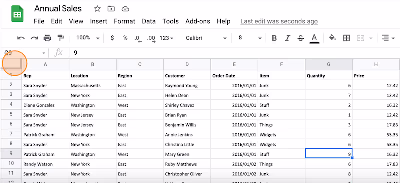
In this example, I'm looking at sales data for North America. Most customers bought multiple products so there are multiple rows of data for each, but I want to see the total spend by customer for the year.
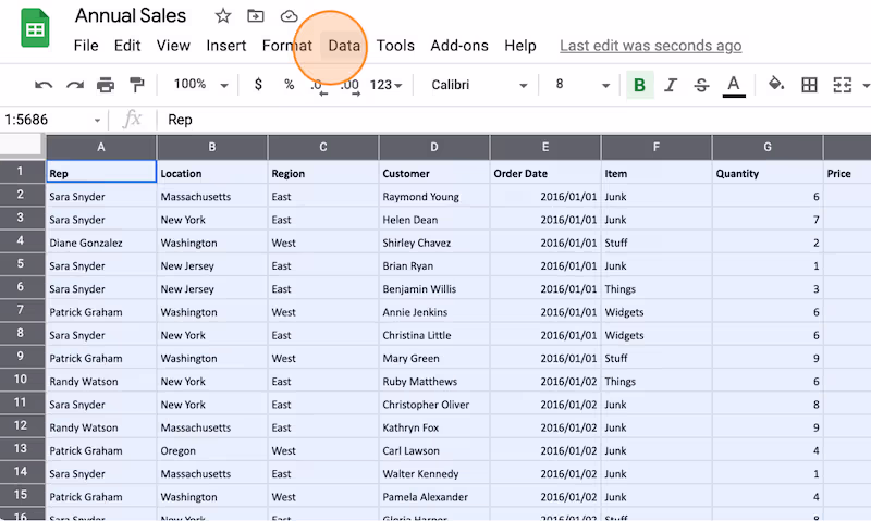
2. Highlight the data set you want to analyze
Highlight the dataset you want to analyze and click "Data." Make sure your data is organized into separate categories.
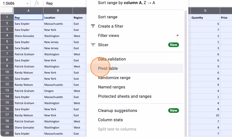
3. Select "Pivot Table"
This will sort through the data you selected.
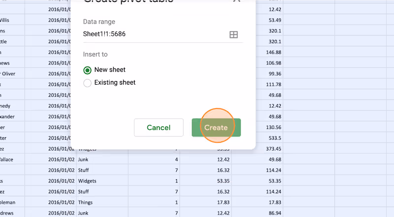
4. Click "Create"
Note that you can create a new sheet or insert the pivot table in the sheet you are on. Make sure to select your preference.
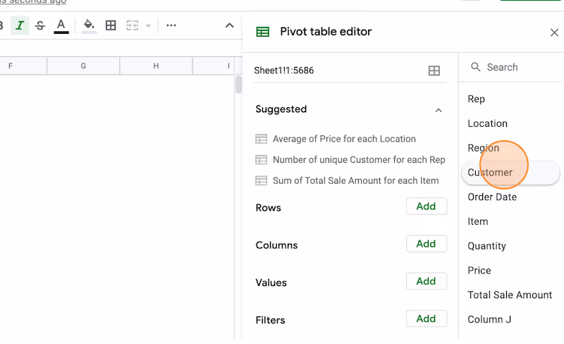
5. Add your data as a "Row"
Select the data you want to analyze and add it as a row in your pivot table. This will let you look at different variables for that data. In this case, I want to see spend by customer. So the "Customer" will be my row.
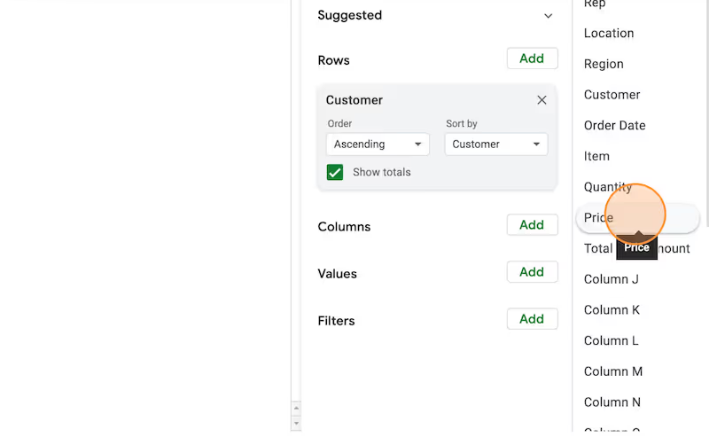
6. Place the value you want to analyze under "Values"
Select the value you want to analyze and place that under "values." In this case, I want to see the total spend by customer so I selected "Price" and place it under "Values."
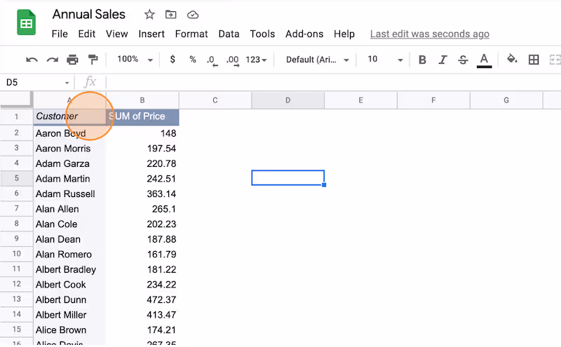
7. Create your pivot table
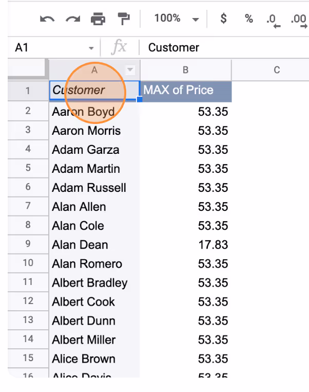
The pivot table then sums the total spend by customer for me. Voila!
Change the operation in a Google Sheets pivot table
By default, pivot tables will "sum" the values, but you can always change the formula. For example, I could look at Max spend. Here's how.
1. Open your pivot table
This will likely be its own sheet in your Google Sheet.
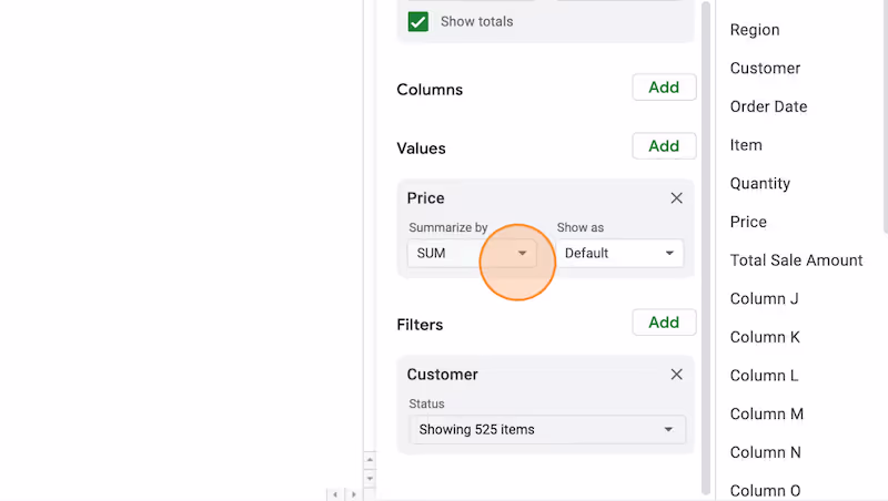
2. Select "Summarize By"
In your pivot table editor, Scroll to the "Values" section and go to the dropdown under "Summarize By."
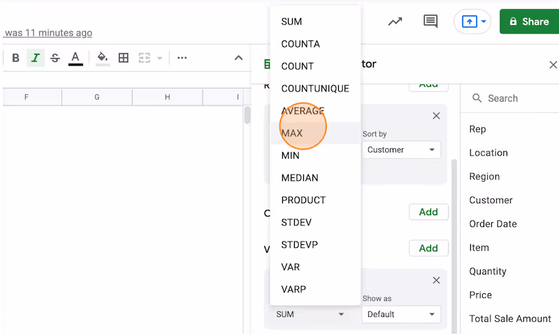
3. Choose the operation you want to use
For example, you might want the average or median of the data. In this example, I'm looking for Max spend, so I'll select MAX.
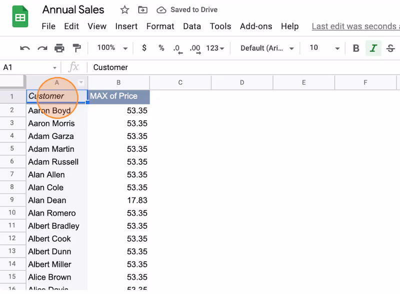
4. Update your pivot table
The pivot table automatically updates to reflect your changes.
Like this step-by-step guide? Check out these related resources
- Google Sheets 101: Google Sheets Tutorial — Everything You Need to Know to Be an Expert
- Free Tool: Google Sheets Training Generator
- Step-by-Step Guide: How to Lock a Row in Google Sheets
- Free Tool: Google Flowchart Generator
- Step-by-step Guide: How to Create a Drop Down in Google Sheets
Get more Google Sheets guides and make your own
Scribe has thousands of guides for Google Sheets, Excel and so much more. Sign up for a free account to save and share this guide with your team.
Scribe is an AI-powered process documentation tool that turns any workflow into a visual step-by-step guide — complete with text, links and annotated screenshots. Build guides for your colleagues and clients in seconds. All for free!

