Google Sheets add and subtract functions

The Google Sheets functions SUM and MINUS are fast and easy ways for you to add and subtract data in your spreadsheet.

SUM formulas in Google Sheets

Basic SUM formula syntax

There are different ways to use the SUM formula based on which cells you want to add.

The basic syntax for the SUM formula is

=SUM(number1, number2, ...)

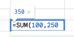
The "numbers" represent the amount that you want to add. For example, if I wanted to add 100 and 250, the formula would be =SUM(100,250)

SUM for a range of cells

More often than not you're using SUM to add up a range of cells in your spreadsheet. The formula for adding up a range is =SUM(range). For example, if I wanted to add up the number in all cells on the 5th row in columns A through D, my formula would look like =SUM(A5:C5).

SUM for combining ranges and single cells

This formula lets you add up ranges of cells AND single cells. For example, if I want to add up a range of cells in row 5, plus a different cell in row 7, I just need to make sure to include the column and row numbers in my breakdown. Here's an example: =SUM(A5:D5,D8)

MINUS formulas in Google Sheets

MINUS formula basic syntax

In Google Sheets, you can subtract values using the MINUS formula. Here's the basic syntax: =MINUS(number1, number2).

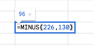
The number stands for the numbers that you wish to subtract from. For example, if I want to know the difference between 226 and 130, I would write =MINUS(226,130)

MINUS formula to subtract cell values

If you want to subtract the difference from one cell to the other, you just need to include the cell names in your formula. For example, if I want to subtract the difference from cell A5 to cell B5, my formula would be =MINUS(A5,B5)

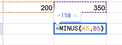
Remember, when using the MINUS formula, the order of the numbers or cell references matters. The first number or reference is the minuend (the number you are subtracting from), and the second number or reference is the subtrahend (the number you are subtracting).

How to add columns in Google Sheets

Here's an example of how to add up all of the values in a single column using the SUM formula.

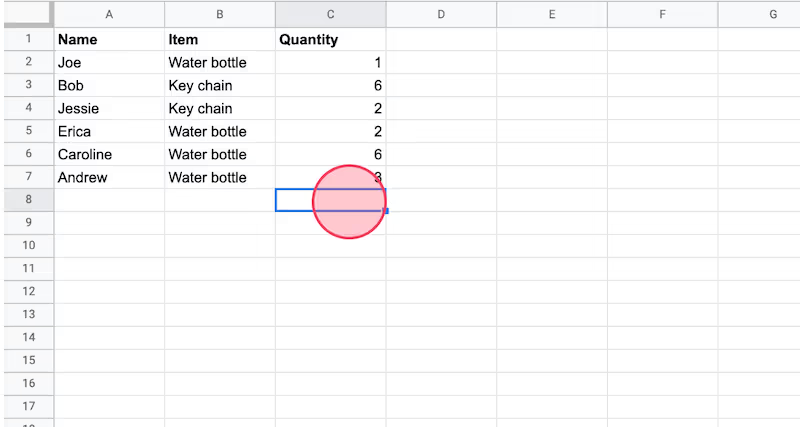
1. Select a cell at the bottom of your column

Scroll to the bottom of your column so you can add the sum below your data.

2. Highlight the column

Use your mouse or press cmd + up (Mac) or ctlr + up (PC) to get to the top of the column you want to add. Type " down" to get to the first cell with data you want to sum, then press cmd + shift + down (Mac) or ctrl + shift + down to select the full set of data you want to sum

‍

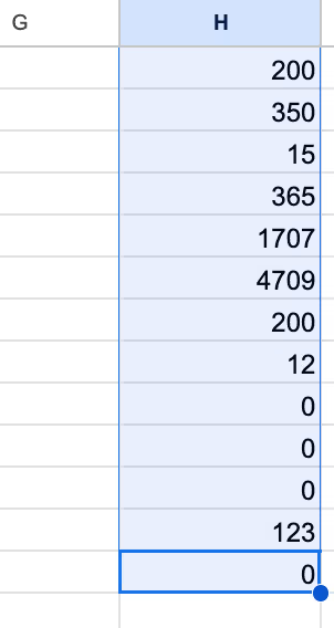
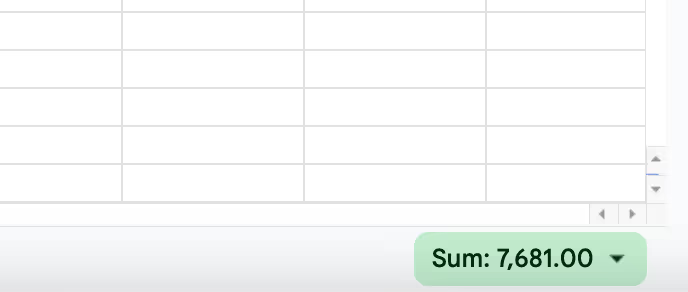
💡Tip: You can also see the sum of your highlighted column at the bottom right of your screen!

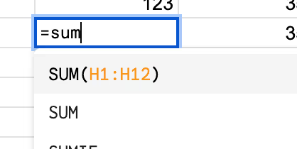
3. Close the formula

Type ")" to close the formula and then type enter, or type in the range of cells you want to add. For example, in this column, we're adding up column H from 1-12, which looks like =SUM(H1:H12).

Like this step-by-step guide? Check out these related resources

• Google Sheets 101: Google Sheets Tutorial — Everything You Need to Know to Be an Expert ‍
• Free Tool: Google Sheets Training Generator‍
• Step-by-Step Guide: How to Lock a Row in Google Sheets
• Free Tool: Google Flowchart Generator
• Step-by-step Guide: How to Create a Drop Down in Google Sheets

Get more Google Sheets guides and make your own

Scribe has thousands of guides for Google Sheets, Excel and so much more. Sign up for a free account to save and share this guide with your team.

Scribe is an AI-powered process documentation tool that turns any workflow into a visual step-by-step guide — complete with text, links and annotated screenshots. Build guides for your colleagues and clients in seconds. All for free!