


How to Freeze, Unfreeze and Merge in Google Sheets
When organizing and sharing data across stakeholders, you want to make that information as clear as possible. By freezing and merging cells, you can make complicated sheets easier to navigate. This helps you present your data more effectively.
For example, you might want to freeze the top row or first column so that headers or labels remain visible as you scroll through a large dataset. And merging cells can be useful for creating headers or titles that span multiple columns or rows, making your spreadsheet more readable and visually appealing.
How to freeze a row in Google Sheets
Freezing a row in Google Sheets comes in handy when you have a large data set, so you can easily understand what data pertains to which category.
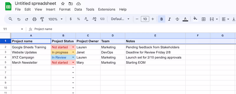
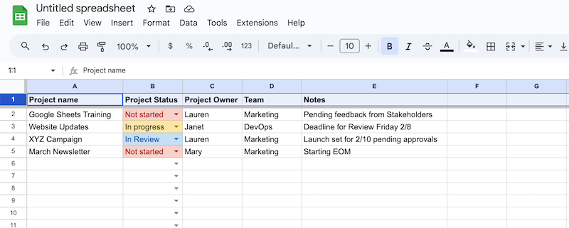
1. Navigate to your Google Sheet
You'll find this sheet in your Google Drive or company's internal wiki.
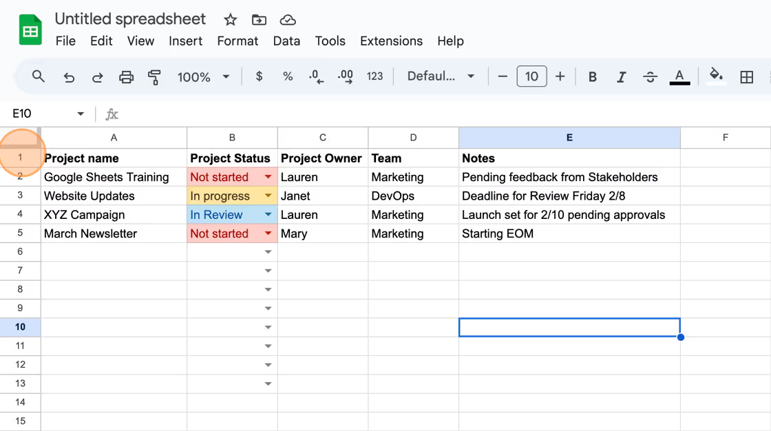
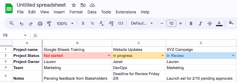
2. Right-click on the row you want to freeze.
This will likely be the top row, depending on your data. By right-clicking, you will highlight the entire row.
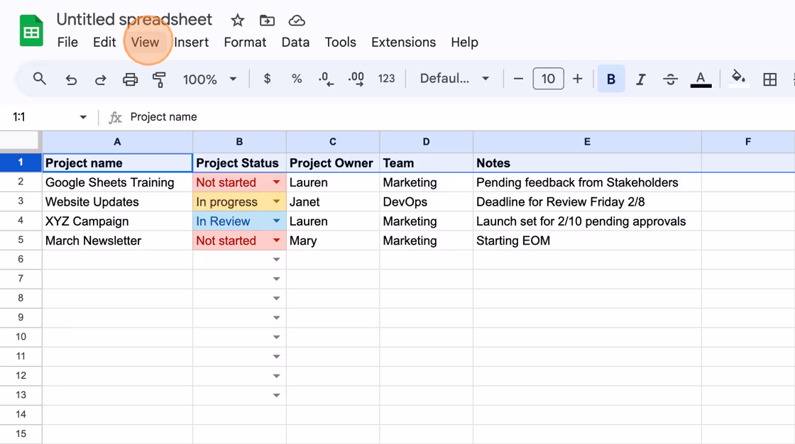
3. Click "View"
Select "View" on the top menu bar.
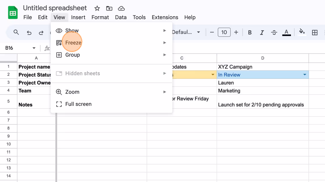
4. Click "Freeze."
Select "Freeze" from the list of options under "View."
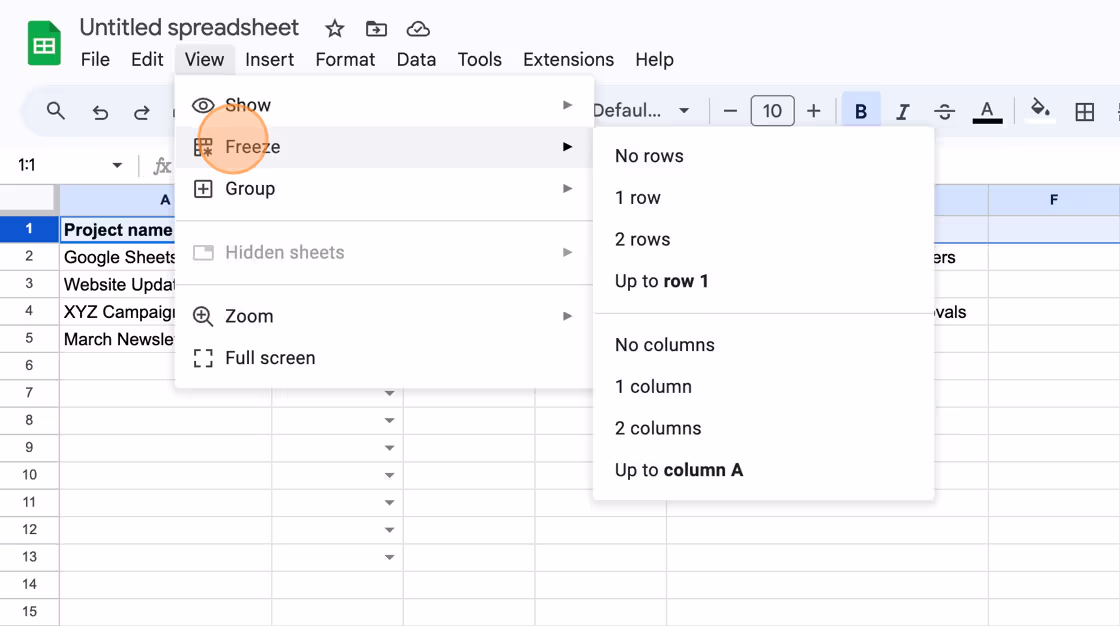
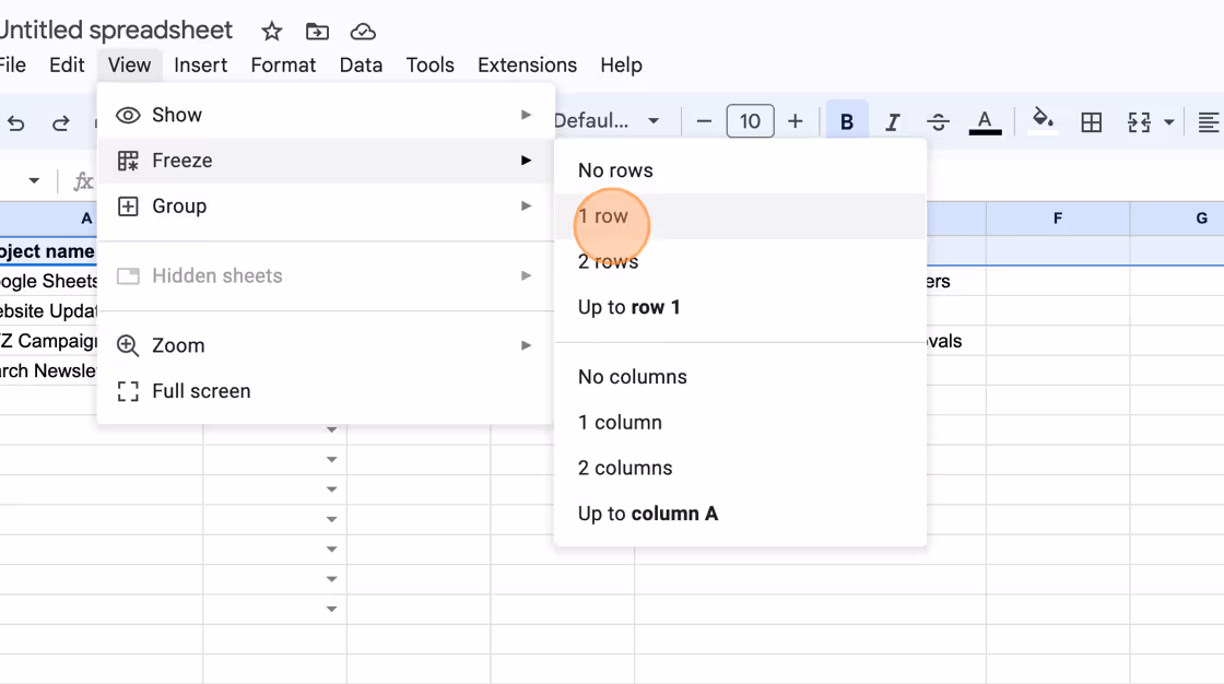
5. Select your row(s).
This menu gives you the option to freeze one row or a set of rows. In this example, we are only freezing row 1. However, depending on the data, you might want to freeze all rows leading up to row 1, or the first two rows.
How to freeze a column in Google Sheets
Depending on how your data is structured, you may need to freeze columns instead of rows in order to more easily navigate your sheet.
1. Navigate to your Google Sheet.
You might have the Google Sheet saved in the drive or your company knowledge base.
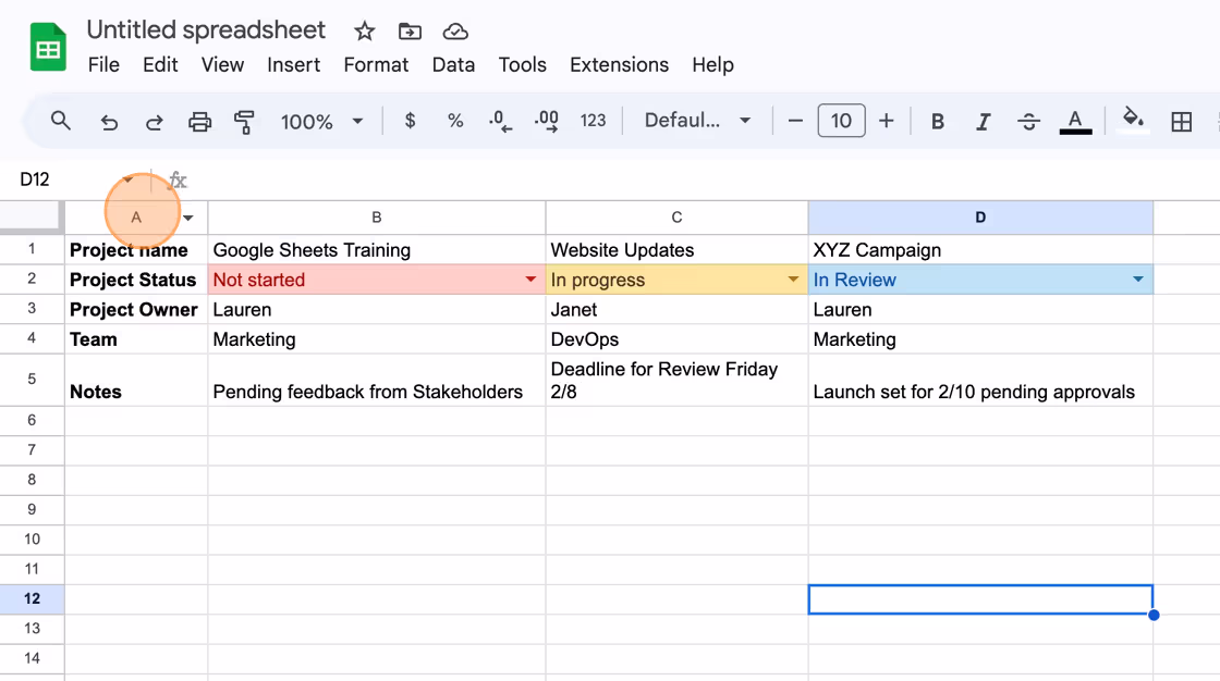
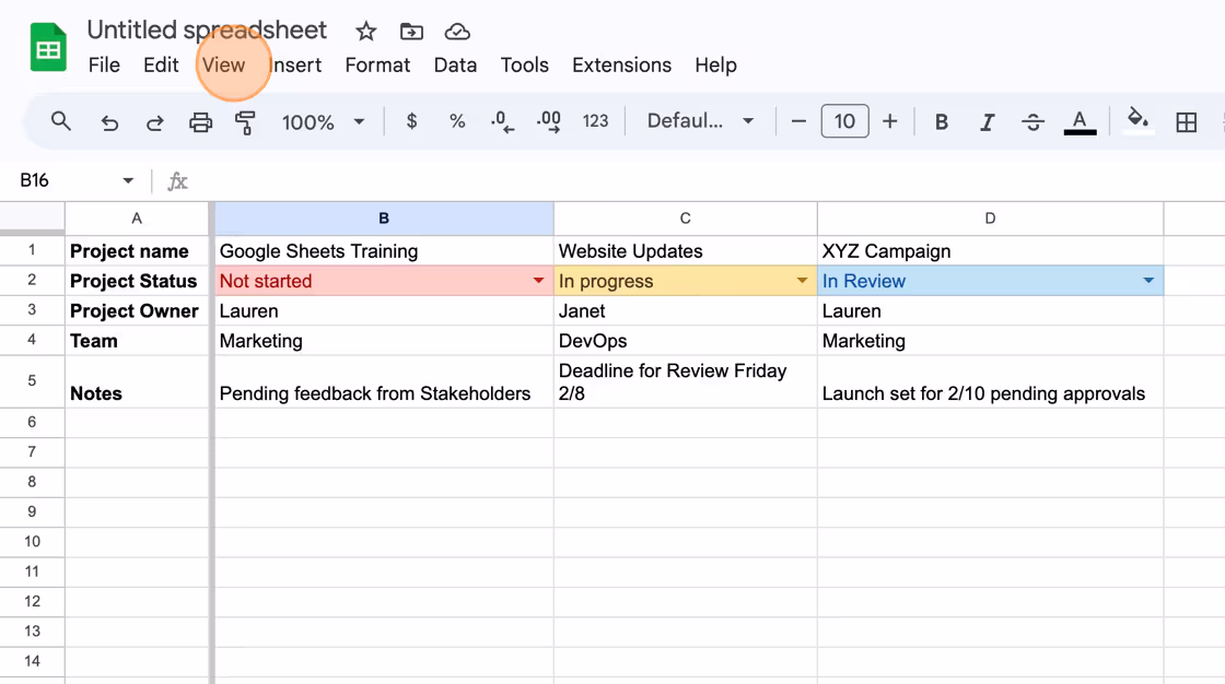
2. Select the column you wish to freeze.
In this example we are choosing "Column A," because it has the topics for content in subsequent columns.
3. Click "View."
Select "View" on the top menu bar.
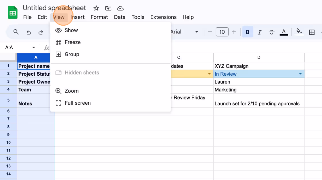
4. Click "Freeze."
Select "Freeze" from the list of options under "View."
5. Select the column(s) you want to freeze.
This menu gives you the option to freeze one column or a set of columns. In this example, we are only freezing column A. However, depending on the data, you might want to freeze all columns leading up your selected column, or the first two columns.

How to unfreeze in Google Sheets
1. Navigate to your Google Sheet.
You might have the Google Sheet saved in the Drive or in your team's knowledge management software.
2. Click "View"
Go to the "View" menu item in your top nav bar.
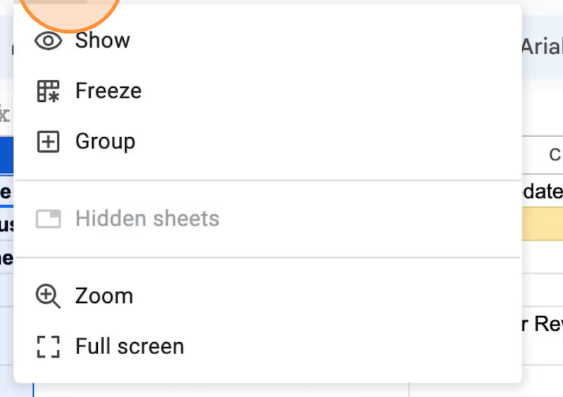
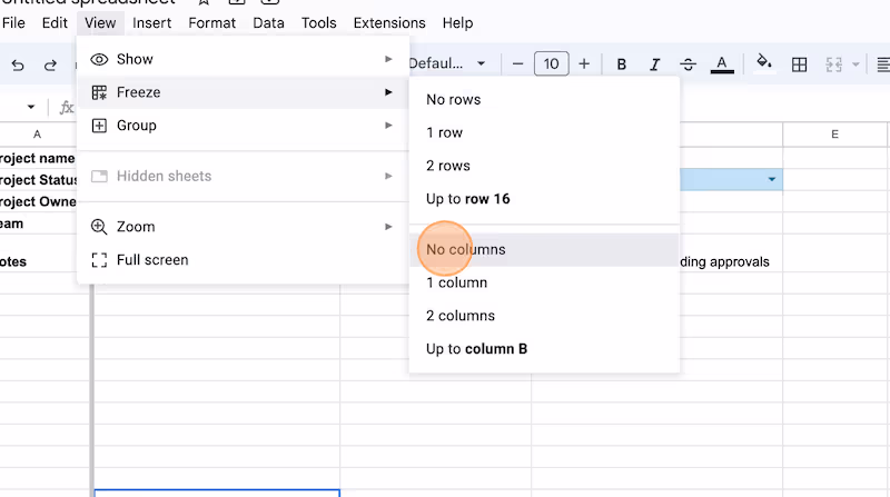
3. Click "Freeze."
This will show you your options for freezing and unfreezing rows and columns.
4. Select "Now Rows" or "No Columns."
Depending on whether you need to unfreeze rows or columns, select the
How to merge cells in Google Sheets
By merging cells in Google Sheets, you can create clear divisions between different sections of your spreadsheet. This can improve the readability of your spreadsheet by reducing clutter and making it easier to focus on important data.
1. Navigate to your Google Sheet.
You might have the Google Sheet saved in the Drive or in your team's process documentation software.
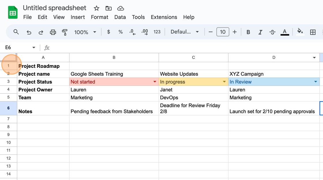
2. Highlight the cells you want to merge.
This may be a group of cells, an entire row or an entire column.

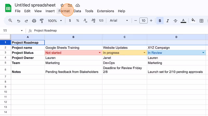
3. Click "Format."
This will be on your top nav bar.
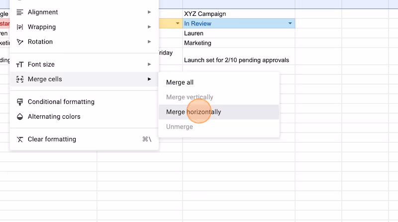
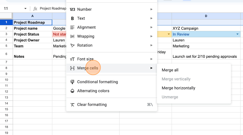
4. Select "Merge Cells."
Scroll to the bottom of the pop-up navigation and hover over "Merge Cells."

5. Select which cells to merge.
Depending on the cells you selected, you can merge horizontally, vertically or all cells.
How to unmerge cells in Google Sheets
Whether you need to manipulate data in individual cells or simplify the data entry process, you may need to unmerge cells in Google Sheets. The process is very similar to when you merger cells.
1. Navigate to your Google Sheet.
You might have the Google Sheet saved in the Drive or in your team's process management software.
2. Select the merged cell.
This may be a row, column or group of cells.
3. Click "Format."
This will be on your top nav bar.
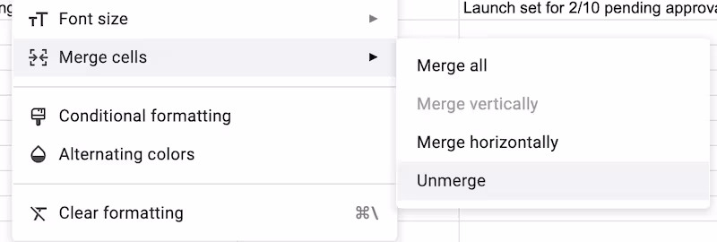
4. Select "Merge Cells."
Scroll to the bottom of the pop-up navigation and hover over "Merge Cells."
5. Click "Unmerge"
This will revert your merged cells into separate cells.
Get more Google Sheets guides and make your own
Scribe has thousands of guides for Google Sheets, Excel and so much more. Sign up for a free account to save and share this guide with your team.
Scribe is an AI-powered process documentation tool that turns any workflow into a visual step-by-step guide — complete with text, links and annotated screenshots. Build guides for your colleagues and clients in seconds. All for free!
Like this guide? Check out these related resources
- Google Sheets 101: Google Sheets Tutorial — Everything You Need to Know to Be an Expert
- Free Tool: Google Sheets Training Generator
- Step-by-Step Guide: How to Lock a Row in Google Sheets
- Free Tool: Google Flowchart Generator
- Step-by-step Guide: How to Create a Drop Down in Google Sheets

